MoRE Developer

This site is under construction.

At first, a description of how to launch the MoRE Developer is given. Then the design of the MoRE Developer user interface is described. The procedure for embedding an alternative spatial basis for modeling, different input data and modeling approaches and for generating results is explained. Furthermore, a short overview of different working tools in MoRE is given.

Launch MoRE

For launching the multi-user version of MoRE, select the respective shortcut (“MoRE_UBA_EN”) in the folder “UBA” or in the folder of a different project. Confirm the execution, if necessary.

For launching the single-user version (SQLite version), select the file “MoRE.exe” in the respective folder.

Reading and writing mode

MoRE starts automatically in reading mode. In this mode, no adjustments can be made except for the interface configuration. To add, edit or delete variables, input data or other items, it is necessary to activate the writing mode. The currently active mode is visible in the lowest bar of the GUI. The mode can be changed from reading to writing (or vice versa) by clicking on the green or yellow button, respectively.

Design of the MoRE Developer GUI

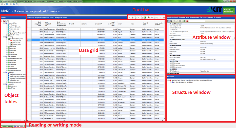
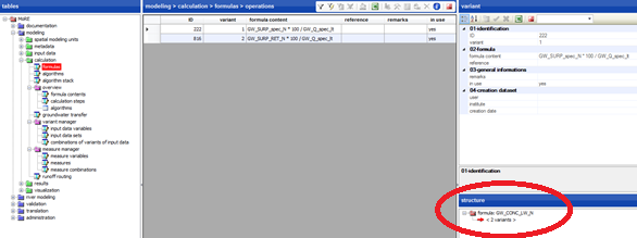
The MoRE Developer GUI consists of the following components:

• Overview of all object tables (left window)
• A data grid (middle window) in which records from a selected object table are displayed
• an attribute window (upper right window) and
• a structure window (lower right window), which both show additional information about a selected record in the data grid.

Further, MoRE features two toolbars with different functionalities (reference) which appear in the title bar of the data grid as well as in the title bar of the attribute window. All mentioned components are explained in detail in the following sections.

Object tables

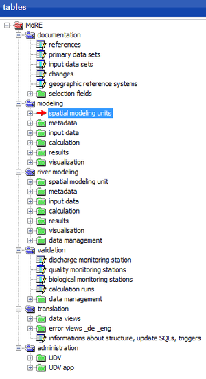
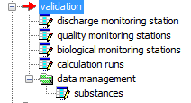
With the MoRE Developer GUI, data from the PostgreSQL-database can be accessed. These data are listed in object tables and summarized in the folders documentation, modeling, validation as well as translation and data management (only visible as administrator). Object tables can be selected by clicking on the name of the desired object table. A red arrow appears in front of the name of the selected object table and the name is highlighted with blue color. Only one object table can be selected at once.

Object table documentation

In the object table documentation, the metadata of the primary data and the input data created from them is managed.

Object table modeling

The object tables modeling contain, first of all, the spatial modeling units as well as the metadata of the variables which are assigned to input data. Additionally, input data values of the variables can be recalled here. In this module all calculation approaches are defined and the created results are shown. Finally, adjustments for the visualization of data in the MoRE Visualizer can be made here. All subunits are explained in detail in the following sections.

Spatial modeling units

The spatial modeling units are the basis for the modeling. At present, analytical units, point sources and planning units are implemented as spatial modeling units.

Analytical units are the primary spatial modeling units, for which eventually all calculations can be made. They are hydrological sub-catchments or e.g. water bodies. In order to model on the level of analytical units, all spatially distributed basic data have to be preprocessed in GIS to mean values or sums. This is especially the case for data which are related to emission pathways with diffuse emission patterns e.g. deposition rates of nitrogen or heavy metals. Pathways which lead to selective emissions can be modeled separately as emissions from point sources. One purpose of this is to avoid inaccuracies that may occur when point sources are first aggregated on the area of analytical units. The detailed acquisition of point sources allows the implementation of purposive measures, e.g. for municipal waste water treatment plants under consideration of their size and processing steps. Besides, improved modeling approaches can be easily included especially for those substances and substance groups which emissions correlate well to point source-specific parameters. Municipal waste water treatment plants, industrial direct dischargers and abandoned mining sites are used for modeling at the moment. Other point sources can be added to MoRE with low effort (Section 3.4.1.2). In Germany, spatial planning units play a major role as a spatial reference of the Water Framework Directive (WFD). They are larger spatial units which are used for the WFD management plants. They are implemented in MoRE and an algorithm was developed, which aggregates the emissions of analytical units to planning unit emissions (Section 3.8).

Metadata

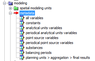
The metadata object table contains information about variables, visualization and literature references. It also contains a change history of the model and the management of preset selection boxes.

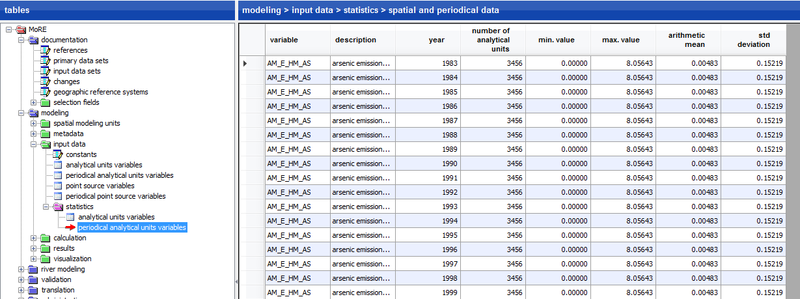
The table all variables lists name, type and reference of all variables and constants as well as the number of formulas they are used in. Variables are classified by their type as constant, spatial, spatial and periodical, point source or periodical point source variables. According to this classification, the variables are listed in separated tables (metadata > constants, metadata > analytical units variables, metadata > periodical analytical units variables, metadata > point source variables and metadata > periodical point source variables) and further attributes like description, family membership, unit, or pathway reference are provided. Besides, an assignment of substances to certain substance groups (metadata > substances) and the allocation of years in balancing periods (metadata > balancing periods) are made. In the submenu planning units > aggregation > final results it can be defined, which results should be aggregated on the level of planning units in order to export the respective results.

Input data

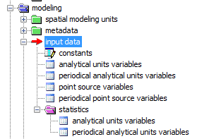
The object table of the input data contains all (preprocessed) data which are necessary for the modeling. They are usually created from primary data, since input data at the level of analytical units or point sources is needed for modeling. Primary data comprise general and substance-specific data, which may be continuous (e.g. digital elevation models) or discrete, regionalized data (e.g. land use, soil type, topography, atmospheric deposition). Sometimes, primary data are only available as point data but are required as regionalized information, which is why an interpolation with geostatistical methods is performed. Some periodically variable primary data may show gaps in the time course such that periodically interpolation methods are needed. If necessary, primary data have to be aggregated (area weighted) in a last step on the basis of the analytical units in a geographic information system. The input data obtained this way can eventually be imported into the database using the graphical user interface MoRE Developer.

Based on the temporal and spatial variability, input data can be arranged in five groups:

• Constant data (constants)
• Data varying in space (analytical units variables)
• Data varying in space and time (periodical analytical units variables)
• Point source specific data (point source variables)
• Point source specific data varying in time (periodical point source variables)

Additionally, MoRE offers the opportunity to statistically analyze analytical units variables as well as periodical analytical units variables. Minimum and maximum as well as the average and the standard deviation are shown as statistical measures in the data grid.

Calculation

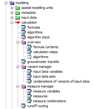
The object table calculation contains the model algorithms for the calculation of emissions into surface waters via different emission pathways. An algorithm stack usually represents a balancing approach for a pathway of water or substance flow e.g. “nitrogen emissions via groundwater”. Each algorithm stack consists of one or more algorithms or algorithm stacks. These algorithms consist of a sequence of calculation steps that are represented by individual formulas (according to these calculation steps). The folder overview contains tables of the formulas, algorithms and algorithm stacks in a more clearly arranged way. More details about the implementation of calculation approaches can be found in section (insert reference). The object table groundwater transfer is also filed here. Further, the variant manager and the measure manager as well as information about the runoff routing are available.

Results

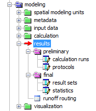
The object table results contains within the subfolder preliminary all generated results as preliminary calculation runs and as a detailed protocol, respectively. In the folder final, all verified results can be stored as results sets as well as statistical data can be found. For management and export of data see the sections ## and ## (add later). Further, the runoff routing model with its bifurcations is shown additionally in this folder.

Visualization

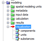
In this object table, tables for components, units and substances are filed. By selecting the components and substances with a checkmark, the user can adjust the visualization.

Object table validation

The object table for validation contains daily discharge values of the stream gauging stations, water quality values of the water monitoring stations and the resulting river loads.

Object table translation and administration

The translation and administration modules are only visible to administrators in the PostgreSQL data base. The river basin management system MoRE was optimized for the use in German and English language. A translation run automatically detects newly implemented expressions which do not have a translation in the MoRE dictionary yet. These expressions have to be translated using the translation module to allow translations from the German to the English version and vice versa. In the administration module, several basic adjustments concerning the database source, structure, attributes and display of the object table, user rights, pre-defined filters, trigger of error messages etc. can be made e.g.

Data grid

By clicking on an object table, its content is displayed in the data grid as a table. The content of the data grid and the heading of the window correspond to the data record selected in the data grid. Clicking on the left margin of the data grid selects a data record in the object table listed. The selected data record is highlighted with blue color. The toolbar enables the use of filters for selecting the data sets.

Attribute window

In the top right window, further details to the selected entries of an object table are displayed. The heading and content of the window correspond to the data record selected in the data grid. New data records may be created and edited in the attribute window.

Structure window

In the bottom right window, the structure of the data record selected in the data grid is displayed. This is especially helpful for the submenu entries from the object table calculation. If the table formulas is selected, the variants of the formulas are displayed in the structure window. If the object table algorithms is selected, the structure window shows the individual calculation steps and if the table algorithm stacks is selected, the individual algorithms are listed. To obtain further details of the shown entries in the structure window, one can click on these entries (< n variants >, < n calculation steps >, < n algorithms >). Then further information is displayed in the data grid.

The structure window is also relevant for the object tables modeling > visualization as well as modeling > spatial modeling units.

MoRE Developer toolbars

In MoRE, two toolbars are implemented which allow interaction with the database as well as creating and editing data records. In addition, the view of the data grid and the attribute window can be adapted. Lists can be exported to Excel. Finally, the calculation can be launched via the toolbar.

Toolbar in the data grid

MoRE has a toolbar in the data grid which offers different tools depending on the object table selected.

These include the following functions:

• filter rows: data records can be filtered by certain criteria
• filter rows by selection: filter data sets by certain criteria within a column
• predefined filter: filter by common selection criteria
• clear filter: previously set filters are removed and all records are shown
• writing table to Excel: exports the content of the data grid to MS Excel
• writing statistics to Excel: exports statistical data on analytical units, planning units and point sources as a table and as diagram to Excel
• tools: execute certain special functions of the calculation engine
• replace: edit or replace several entries at the same time
• delete selected rows: delete a data set

If a tool is available or not (then shown grayed out) depends on the object table selected. Via the special function TOOLS, different functionalities are available in the individual object tables.

Toolbar in the attribute window

In the attribute window, another toolbar is implemented. This toolbar includes the following functions:

• categorized: arrange the entries in the attribute window
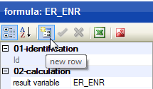
• new row: create, accept or discard new data sets
• writing properties to Excel: export the content of the attribute window
• documents: upload pdf-Documents related to the data sets

Toolbar in the title bar

The toolbar in the title bar contains the following tools:

• open parameter database: Developer’s tool with access to the data base (not available for users due to password protection)
• check parameters: SQL, which fill tables, check and update data types if necessary
• rebuild tree structure of tables: updates the tree structure view
• logged in as administrator: allows to log in as administrator, if the admin entity of the model is used
• about MoRE: Information about version and development of MoRE
• MoRE manual: The current manual is opened as a PDF file

Some of these tools are only available, when the user is logged in as administrator. Unavailable tools are shown grayed out.

Implementaion of input data and modeling approaches

Using MoRE Developer, one can calculate emissions and river loads for both already implemented analytical units with the standard input data and modeling approaches or with other analytical units and point sources. If other (often more detailed) input data are available, these can be imported to MoRE and used as a variant of input data for modeling. Depending on the data basis, modeling approaches may be adjusted and stored as a variant next to the basic variant. Thus, this allows calculating emissions via a pathway in different variations with distinct input data sets or diverse modeling approaches. The achieved results can be compared to evaluate the quality of the input data and modeling approaches.

Implementing a spatial basis for modeling

Implementing new analytical units

If another spatial basis for modeling aside from the one already embedded is desired, other analytical units have to be implemented in MoRE. For example, smaller units as well as river basin districts outside of Central Europe can be embedded. First, these new hydrological catchments have to be derived via a GIS routine (e.g. ArcHydro or other watershed delineation tools). The import of new analytical units works similar to the import of input data.

Preparation of the import files in Excel

For the import of input data to MoRE a template file is available (“MoRE_import.xls”), which is delivered with the system. The file contains a spreadsheet for the import of the catchments (“analytical units”).

Import into the system

If the object table modeling > spatial modeling units > analytical units is selected, new analytical units can be integrated in MoRE via the special function in the toolbar of the data grid (TOOLS → INPUT DATA → IMPORT) by choosing the prepared Excel file. The box “overwriting existing values” is checked by default. By clicking on “start data import”, the data are imported. Please note: Analytical units in MoRE may be deleted from the object table spatial modeling units > analytical units using the tool DELETE SELECTED ROWS. If necessary, the stored input data have to be deleted additionally from the object table input data > analytical unit variables or input data > periodical analytical unit variables (TOOLS → MORE → DELETE INPUT DATA)

Creating a new runoff routing model

All calculations in MoRE are performed on the level of analytical units. For the aggregation of river loads within the water system, a runoff routing model is needed. It represents the flow direction of every individual analytical unit (for further details see Fuchs et al. (2010) , S.8). To derive a runoff routing model, every analytical unit has to be assigned a downstream analytical unit. Usually this is done in a preprocessing. If so, the runoff routing model might exist as a spreadsheet file, which can be imported into MoRE. Sometimes it may occur that one analytical unit drains into two different downstream analytical units (e.g. when there are channels). For this case, the field ”Id Split” was created. This field shows the ID of the second downstream analytical unit in case of a branching (“splitting”). If there is no branching, the field remains empty. In order to distribute the proportions onto the two downstream analytical units, the variable RM_FCT_Q_SPLIT was introduced. When calculating the load along the runoff routing, the load is multiplied in the case of a first-order branching with (1 - RM_FCT_Q_SPLIT) and in the case of a second-order branching with RM_FCT_Q_SPLIT. When dealing with a small number of changes of already existing analytical units, these changes may be done manually in the object table spatial modeling units > analytical units. For manual entries, the writing mode has to be active. Then, the respective areas are selected in the columns “ID of downstream analytical unit”and “ID split”.

If a different topology should be used for modeling, this has to be imported in MoRE first. For this, the topology has to be saved in the import template file (spreadsheet “analytical units”) and subsequently imported in MoRE. At least one analytical unit has to be selected for creating the new runoff routing model via the special function TOOLS → RUNOFF ROUTING → CALCULATE. The result will be shown in the object table results > runoff routing.

Implementing new point sources

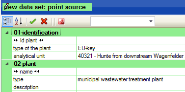
The point sources are entered in the object table modeling > spatial modeling units > point sources. There are two options for implementation of point sources. The first option is a manual entry by activating the writing mode and creating a new data set in the attribute window . The “ID” and the “type” of point source are mandatory fields. Necessarily, the analytical unit has to be selected, in which the point source is located.

In order to start the calculation run for a point source, it is essential to define a validity period. Please note the syntax of the validity. The starting and terminal year are separated by a hyphen, individual years are separated using commas. This way of implementing a point source is applicable, when individual plants should be added to the entire data collective.

Syntax of the validity period for point sources.

Id plant	...	validity
1	...	2006-2011
2	...	2006-2009, 2011
3	...	2006, 2008-2009, 2011

When there are no data in the system yet and a long list of point sources has to be imported, the implementation should be performed using the special function TOOLS → IMPORT INPUT DATA in the object table spatial modeling unit > point sources. For this purpose, the spreadsheet “point sources” of the import template file must be filled and imported. The import of point sources works similar to the import of analytical units. Filling the columns “id point sources”, “type of point source”, “validity” and “ID of analytical unit” is mandatory.

Create new data sets

The basic procedure for creating new data sets is as follows:

1. Activate the writing mode
2. Select the according object table in the left window. It will become visible in the data grid.
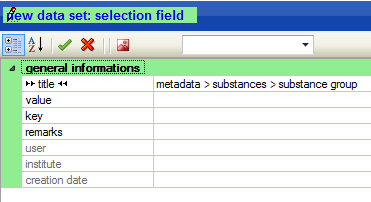
3. Create a new data set using the toolbar of the attribute window.

   

4. Fill in all needed information.
5. If applicable, attach documents with additional information, e.g. flow charts showing the calculation steps, excel files, R-scripts or papers.

   

6. Transfer the data record to the database or discard the record.

   

   

Implement new input data in MoRE

Before implementing new input data in MoRE, the respective variables have to be created in the system. Subsequently, the input data can be imported to MoRE. New substances, substance groups or units have to be added to MoRE before the variables are created to enable the correct assignment. Further metadata of the variables can be added the same way as substance groups and units are added in the object table documentation (e.g. components, emission pathways – here as specification or parameter).

Creating new substances groups and substances

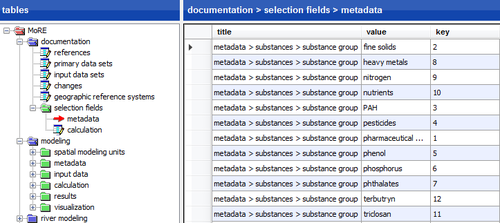
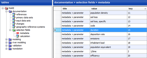
New substance groups can be added as a new data set in the object table documentation > selection fields > metadata. In the data grid all previously entered substance groups are shown in the column “title” under the term “metadata > substances > substance group”.

By adding a new data set, a new substance group can be created. Please note that the name of the new substance group is entered under “value” and a unique “key” is provided e.g. as a consecutive numbering.

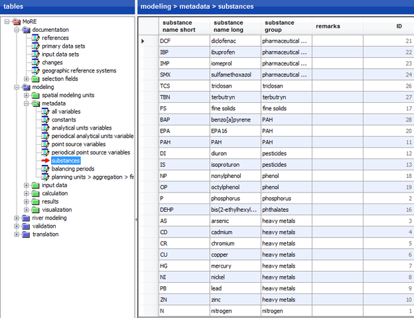
Subsequently, the new substances belonging to the substance group can be added in the object table modeling > metadata > substances. Please note that “substance name short” can only contain upper- and lower case letters. The ID of the substance is automatically complemented by a consecutive numbering.

Creating a new unit

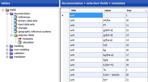
Within the object table documentation > selection fields > metadata, a unit can be created following the routine described above for substance groups. Enter the word “unit” as the “title” and the actual unit as “value”. Please note to provide a unique “key”, e.g. as a consecutive numbering.

Creating new parameter

Using the object table documentation > selection fields > metadata, a parameter can be created following the routine described above for substance groups. Enter the term “metadata > parameter” as the “title” and the actual parameter as “value”. Please note to provide a unique “key”, e.g. as a consecutive numbering.

References

- ↑ [1] Fuchs, S., Scherer, U., Wander, R., Behrendt, H., Venohr, M., Opitz, D., Hillenbrand, Th., Marscheider-Weidemann, F., Götz, Th. (2010): Berechnung von Stoffeinträgen in die Fließgewässer Deutschlands mit dem Modell MONERIS. Nährstoffe, Schwermetalle und Polyzyklische aromatische Kohlenwasserstoffe. UBA-Texte 45/2010, Dessau